概率论 Probability Theory

Basics

Definition: Let $I \subseteq \mathbb{R}$. Let $X_t : \Omega \to \mathbb{R}, t\in I$, be random variables on the same probability space $(\Omega. \mathcal{F}, P)$. Then $X = (X_t)_{t \in I}$ is called a real-valued stochastic process.

Expected value / Expectation / Erwartungswert / 期望

Definition : Let $X$ be a random variable on a probability space $(\Omega,\mathcal{F},P)$. The expectation of $X$ is defined by

$\mathbb{E}[X] = \int_{\Omega}X(\omega)P(d\omega).$

Theorem: Let $X:\Omega \to S$ be a random variable on a probability space $(\Omega,\mathcal{F},P)$ with distribution $\mu$ and let $g:S\to \mathbb{R}$ be a measurable function. Then

$\mathbb{E}[g(X)] = \int_{S}g(x)\mu(dx).$

Corollary: If $X$ is a discrete random variable with values in $S$, then

$\mathbb{E}[g(X)] = \sum_{x \in S}g(x)P(X=x).$

Corollary: If $X$ is a discrete random variable with values in $S \subseteq \mathbb{R}$, then

$\mathbb{E}[X] = \sum_{x \in S}xP(X=x).$

Proof: Choose $g = id_S: S \to S \subseteq \mathbb{R}$.$\square$

Corollary: If $X : \Omega \to \mathbb{R}^n$ has the probability density function (Verteilungsdichte) $f$, then for every Borel-measurable function $g : \mathbb{R}^n \to \mathbb{R}$, the following holds:

$\mathbb{E}[g(X)] = \int_{\mathbb{R}^n} g(x) f(x) \, dx.$

Corollary: If $X$ has values in $\mathbb{R}$

$\mathbb{E}[X] = \int_{\mathbb{R}} x f(x) \, dx.$

Theorem (Linearity): Let $X,Y :\Omega \to \mathbb{R}$ be random variables in $\mathcal{L}^1$. Then

$\mathbb{E}[aX+bY] = a\mathbb{E}[X] + b\mathbb{E}[Y] \ \ \text{ for all }a,b \in \mathbb{R}$

Theorem: Let$X,Y :\Omega \to \mathbb{R}$be independent random variables, $g,h: \mathbb{R} \to \mathbb{R}$ be Borel-measurable function with $E[|g(X)|], E[|h(Y)|] < \infty$. Then

$\mathbb{E}[g(X)h(Y)] = \mathbb{E}[g(X)] \mathbb{E}[h(Y)].$

proof: Since $X$ and $Y$ are independent, the joint distribution of $(X, Y)$ is the product of the marginal distributions $P_X \times P_Y$. Using Fubini’s theorem, we obtain

$\begin{align*} \mathbb{E}[g(X)h(Y)] &= \int_{\mathbb{R}} \int_{\mathbb{R}} g(x)h(y) \, P_X(dx) P_Y(dy)\\ &= \left( \int_{\mathbb{R}} g(x) \, P_X(dx) \right) \left( \int_{\mathbb{R}} h(y) \, P_Y(dy) \right) = \mathbb{E}[g(X)] \mathbb{E}[h(Y)]. \end{align*}$

$\square$

Corollary: Let$X,Y :\Omega \to \mathbb{R}$be independent random variables in $\mathcal{L}^1$, then

$\mathbb{E}[XY] = \mathbb{E}[X] \mathbb{E}[Y].$

Moment

Definition : $E[X^n]$is called the $n^{\text{th}}$ moment of X.

Theorem:

Let $X \sim \mathcal{N}(\mu,\sigma^2)$ be a random variable. Then for any non-negative integer $p$ we have:

$\mathbb{E}[(X - \mu)^p] =\begin{cases}0 & \text{if } p \text{ is odd}, \\\sigma^p (p - 1)!! & \text{if } p \text{ is even}.\end{cases}$

Here, $n!!$ denotes the double factorial, that is, the product of all numbers from $n$ to 1 that have the same parity as $n$.

Corollary:

Let $X \sim \mathcal{N}(0,\sigma^2)$ be a random variable. Then for any non-negative integer $p$ we have:

$\mathbb{E}[X^p] =\begin{cases}0 & \text{if } p \text{ is odd}, \\\sigma^p (p - 1)!! & \text{if } p \text{ is even}.\end{cases}$

Example:

Let $X \sim \mathcal{N}(0,\sigma^2)$ be a random variable, we have:

$\mathbb{E}[X^2] = \sigma^2$
$\mathbb{E}[X^3] = 0$
$\mathbb{E}[X^4] = 3 \sigma^4$

Variance / Varianz / 方差

Definition: Let$X\in \mathcal{L}^1$. Then

$\text{Var}(X) = \mathbb{E}[(X-\mathbb{E}(X))^2]$

is called the variance of$X$and

$\sigma_X = \sqrt{Var(X)}$

is the standard deviation of $X$.

Theorem: Let$X\in \mathcal{L}^1$, then

$\text{Var}(X) = \mathbb{E}[X^2] - \mathbb{E}[X]^2.$

proof:

let $\mu:=E[X]$.

$\begin{align*} \text{Var}(X) &= \mathbb{E}[(X-\mu)^2]\\ &= \mathbb{E}[X^2-2\mu X + \mu^2]\\ &= \mathbb{E}[X^2]-2\mu E[X] + \mu^2\\ &= \mathbb{E}[X^2]- \mu^2 \end{align*}$

$\square$

Theorem: Let $X$ be a random variable with finite expectation. For $a,b \in \mathbb{R}$, it holds that:

$\text{Var}(aX + b) = a^2 \text{Var}(X)$

proof:

$\begin{align*} \text{Var}(aX + b) &= \mathbb{E}\left[(aX + b - \mathbb{E}[aX+b])^2\right] \\ &= \mathbb{E}\left[(aX + b - (a\mathbb{E}[X] + b))^2\right] \quad \text{(by linearity)}\\ &= \mathbb{E}\left[a^2 (X - \mathbb{E}[X])^2\right] \\ &= a^2 \text{Var}(X) \end{align*}$

$\square$

Theorem: Let $X,Y$ be independent random variables, then

$\text{Var}(X + Y) = \text{Var}(X) + \text{Var}(Y)$

proof:

$\begin{align*} \text{Var}(X + Y) &= \mathbb{E}[(X+Y)^2] - \mathbb{E}[X+Y]^2 \\ &= \mathbb{E}[X^2] + \mathbb{E}[Y^2] - \mathbb{E}[X]^2 - \mathbb{E}[Y^2] \quad \text{(by independence)}\\ &= \text{Var}(X) + \text{Var}(Y) \end{align*}$

$\square$

Theorem:

Let $X,Y$ be independent random variables, then

$Var(XY) = Var(X)Var(Y) + Var(X)\mathbb{E}[Y]^2 + Var(Y)\mathbb{E}[X]^2$

Proof:

$\begin{align*} Var(XY) &= \mathbb{E}[X^2Y^2] - \mathbb{E}[XY]^2\\ &=\mathbb{E}[X^2]\mathbb{E}[Y^2] - \mathbb{E}[X]^2\mathbb{E}[Y]^2\\ &= (Var(X) + \mathbb{E}[X]^2)(Var(Y) + \mathbb{E}[Y]^2) - \mathbb{E}[X]^2\mathbb{E}[Y]^2\\ &= Var(X)Var(Y) + Var(X)\mathbb{E}[Y]^2 + Var(Y)\mathbb{E}[X]^2 \end{align*}$

. $\square$

Covariance / 协方差

Definition :For real-valued random variables$X, Y \in L^2$, the covariance of$X$and$Y$is defined by

$\text{Cov}(X, Y) = \mathbb{E}\Bigl[(X - \mathbb{E}[X])(Y - \mathbb{E}[Y])\Bigl]$

Theorem:
(a) $\text{Cov}(X, X) = \text{Var}(X)$

(b) $\text{Cov}(X, Y) = \mathbb{E}[XY] - \mathbb{E}[X]\mathbb{E}[Y]$

Proof:

(a) Clear from the definition.

(b) By the linearity of expectation, it follows:

$\text{Cov}(X, Y) = \mathbb{E}[XY - X\mathbb{E}[Y] - \mathbb{E}[X]Y + \mathbb{E}[X]\mathbb{E}[Y]] = \mathbb{E}[XY] - \mathbb{E}[X]\mathbb{E}[Y].$

Theorem: Let $X_i, Y_j \in L^2$, $a_i, b_j \in \mathbb{R}$, $1 \leq i \leq n$, $1 \leq j \leq m$. Then:

(a) The covariance is bilinear:

$\operatorname{Cov}\left( \sum_{i=1}^{n} a_i X_i, \sum_{j=1}^{m} b_j Y_j \right) = \sum_{i=1}^{n} \sum_{j=1}^{m} a_i b_j \operatorname{Cov}(X_i, Y_j)$

(b)

$\operatorname{Var}\left( \sum_{i=1}^{n} X_i \right) = \sum_{i=1}^{n} \operatorname{Var}(X_i) + \sum_{\substack{i,j=1\\i \neq j}}^{n} \operatorname{Cov}(X_i, X_j)$

In particular:

$\operatorname{Var}(X_1 + X_2) = \operatorname{Var}(X_1) + \operatorname{Var}(X_2) + 2 \operatorname{Cov}(X_1, X_2)$

$\operatorname{Var}\left( \sum_{i=1}^{n} X_i \right) = \sum_{i=1}^{n} \operatorname{Var}(X_i)$

This holds especially if $X_1, \dots, X_n$ are independent.

Proof:

(a) Since $\operatorname{Cov}(X, Y) = \operatorname{Cov}(Y, X)$, it suffices to show linearity in the first argument. From the linearity of expectation, it follows:

$\begin{align*} \operatorname{Cov}\left( \sum_{i=1}^{n} a_i X_i, Y \right) &= \mathbb{E}\left[ \left( \sum_{i=1}^{n} a_i X_i - \mathbb{E}\left[ \sum_{i=1}^{n} a_i X_i \right] \right)(Y - \mathbb{E}[Y]) \right] \\ &= \mathbb{E}\left[ \sum_{i=1}^{n} a_i (X_i - \mathbb{E}[X_i])(Y - \mathbb{E}[Y]) \right] = \sum_{i=1}^{n} a_i \operatorname{Cov}(X_i, Y) \end{align*}$

(b) Using part (a), we get:

$\begin{align*} \operatorname{Var}\left( \sum_{i=1}^{n} X_i \right) &= \operatorname{Cov}\left( \sum_{i=1}^{n} X_i, \sum_{j=1}^{n} X_j \right) = \sum_{i=1}^{n} \sum_{j=1}^{n} \operatorname{Cov}(X_i, X_j) \\ &= \sum_{i=1}^{n} \operatorname{Var}(X_i) + \sum_{\substack{i,j=1\\i \neq j}}^{n} \operatorname{Cov}(X_i, X_j) \end{align*}$

In the special case $n = 2$, this gives:

$\operatorname{Var}(X_1 + X_2) = \operatorname{Var}(X_1) + \operatorname{Var}(X_2) + \operatorname{Cov}(X_1, X_2) + \operatorname{Cov}(X_2, X_1)$

Moment generating function

Definition: Let $X$ be a random variable such that $\mathbb{E}[e^{tX}] < \infty$, then the moment generating function is defined as

$M_X(t) := \mathbb{E}[e^{tX}].$

for all $t \in \mathbb{R}$.

Theorem: Let $X \sim N(\mu,\sigma^2)$, then the moment generating function exists and is equal to

$M_X(t) = e^{\mu t + \frac{\sigma^2 t^2}{2}}.$

Clearly, if $X \sim N(0,1)$, we have

$M_X(t) = e^{\frac{t^2}{2}}.$

Proof:

Let $X \sim N(\mu,\sigma^2)$, and

$f(x) := \frac{1}{\sqrt{2\pi} \sigma} e^{-\frac{(x - \mu)^2}{2\sigma^2}}$

be its density function. Then, by definition we have

$\begin{align*} M_X(t) = \mathbb{E}[e^{tX}] &= \frac{1}{\sqrt{2\pi}\sigma} \int_{-\infty}^{\infty} e^{tx} \cdot e^{- \frac{(x - \mu)^2}{2\sigma^2}}\, dx \\ &= \frac{1}{\sqrt{2\pi}\sigma} \int_{-\infty}^{\infty} \exp\left(tx - \frac{(x - \mu)^2}{2\sigma^2} \right)\, dx \end{align*}$

Notice that

$\begin{align*} tx - \frac{(x - \mu)^2}{2\sigma^2} &= tx - \frac{1}{2\sigma^2}(x^2 - 2\mu x + \mu^2) \\ &= tx - \frac{x^2}{2\sigma^2} + \frac{\mu x}{\sigma^2} - \frac{\mu^2}{2\sigma^2} \\ &= -\frac{1}{2\sigma^2}x^2 + \left(t + \frac{\mu}{\sigma^2}\right)x - \frac{\mu^2}{2\sigma^2} \\ &= -\frac{1}{2\sigma^2} \left[ x^2 - 2\sigma^2 \left(t + \frac{\mu}{\sigma^2}\right)x \right] - \frac{\mu^2}{2\sigma^2} \\ &= -\frac{1}{2\sigma^2} \left[ x^2 - 2(\mu + \sigma^2 t)x \right] - \frac{\mu^2}{2\sigma^2} \\ &= -\frac{1}{2\sigma^2} \left[ x^2 - 2(\mu + \sigma^2 t)x + (\mu + \sigma^2 t)^2 - (\mu + \sigma^2 t)^2 \right] - \frac{\mu^2}{2\sigma^2} \\ &= -\frac{1}{2\sigma^2} \left[ (x - \mu - \sigma^2 t)^2 - (\mu + \sigma^2 t)^2 \right] - \frac{\mu^2}{2\sigma^2} \\ &= -\frac{(x - \mu - \sigma^2 t)^2}{2\sigma^2} + \frac{(\mu + \sigma^2 t)^2 - \mu^2}{2\sigma^2} \\ &= -\frac{(x - \mu - \sigma^2 t)^2}{2\sigma^2} + \mu t + \frac{1}{2} \sigma^2 t^2 \end{align*}$

Then we have

$\begin{align*} M_X(t) &= \frac{1}{\sqrt{2\pi}\sigma} \int_{-\infty}^{\infty} \exp\left( -\frac{(x - \mu - \sigma^2 t)^2}{2\sigma^2} + \mu t + \frac{1}{2} \sigma^2 t^2 \right)\, dx \\ &=e^{\mu t + \frac{1}{2} \sigma^2 t^2} \cdot \frac{1}{\sqrt{2\pi}\sigma} \int_{-\infty}^{\infty} \exp\left( -\frac{(x - \mu - \sigma^2 t)^2}{2\sigma^2} \right)\, dx \\ &= e^{\mu t + \frac{\sigma^2 t^2}{2}}. \end{align*}$

p.s.: the calculation/proof of Gaussian integral

$\frac{1}{\sqrt{2\pi}\sigma} \int_{-\infty}^{\infty} \exp\left( -\frac{(x - \mu - \sigma^2 t)^2}{2\sigma^2} \right)\, dx = \frac{1}{\sqrt{2\pi}} \int_{-\infty}^{\infty} e^{-\frac{y^2}{2}}\, dy = 1$

can be found here:

https://archer-baiyi.github.io/2025/06/26/TUM%20%20%E6%95%B0%E5%AD%A6%20%E7%AC%94%E8%AE%B0/%E6%A6%82%E7%8E%87%E8%AE%BA/Probability-Distributions/#Normal-Distribution

.$\square$

Important Inequalities

Theorem (Jensen's Inequality):

Let $\varphi:\mathbb{R} \to \mathbb{R}$ be convex. If $\mathbb{E}[|X|] < \infty$, then $\mathbb{E}[\varphi(X)]$ is well-defined and one has

$\varphi(\mathbb{E}[X]) \leq \mathbb{E}[\varphi(X)].$

Corollary:

$|\mathbb{E}[X]| \leq \mathbb{E}[|X|]$

2. for $p \geq 1 :$

$|\mathbb{E}[X]|^p \leq \mathbb{E}[|X|^p]$

3. for $1 \leq p < q :$

$(\mathbb{E}[|X|^p])^{\frac{1}{p}} \leq (\mathbb{E}[|X|^q])^{\frac{1}{q}}$

proof:

1. take $\varphi(x) = |x|$.

2. take $\varphi(x) = |x|^p, p \geq 1$.

3. Let $1 \leq p < q , \alpha := q/p > 1, Z := |X|^p$. From 2 we have

$\begin{align*} &\quad |\mathbb{E}[Z]|^\alpha \leq \mathbb{E}[|Z|^\alpha] \\ \Longleftrightarrow &\quad |\mathbb{E}[|X|^p]|^\alpha \leq \mathbb{E}[|X|^{\alpha p}] \\ \Longleftrightarrow &\quad |\mathbb{E}[|X|^p]|^{\frac{1}{p}} \leq \mathbb{E}[|X|^{\alpha p}]^{\frac{1}{\alpha p}} \\ \Longleftrightarrow &\quad (\mathbb{E}[|X|^p])^{\frac{1}{p}} \leq (\mathbb{E}[|X|^q])^{\frac{1}{q}} \end{align*}$

$\square$

Theorem (Markov's inequality):

Let $X$ be a real-valued random variable and let $f : [0, \infty) \to [0, \infty)$ be a monotonically increasing function with $f(x) > 0$ for all $x > 0$.
Then for all $a > 0$ we have:

$P(|X| \geq a) \leq \frac{\mathbb{E}[f(|X|)]}{f(a)}.$

In particular, for all $a, p > 0$, it holds:

$P(|X| \geq a) \leq \frac{\mathbb{E}[|X|^p]}{a^p}.$

Proof:

Since $f \geq 0$ and is monotonically increasing, we have :

$f(|X|) \geq f(|X|)\mathbf{1}_{\{|X| \geq a\}} \geq f(a)\mathbf{1}_{\{|X| \geq a\}}.$

From the monotonicity of the expectation, it follows that:

$\mathbb{E}[f(|X|)] \geq \mathbb{E}[f(a)\mathbf{1}_{\{|X| \geq a\}}] = f(a)P(|X| \geq a).$

Since $f(a) > 0$, the claim follows. $\square$

Theorem (Chebyshev's inequality):

Let $X \in \mathcal{L}^2$ (i.e.$\mathbb{E}[|X|^2] < \infty$) be a real-valued random variable, then for all $a > 0$ we have:

$P(|X-\mathbb{E}[X]| \geq a) \leq \frac{\text{Var}(X)}{a^2}.$

Proof:

Let $Y = X-\mathbb{E}[X]$, $f(x):=x^2$. By applying Markov’s inequality we have:

$P(|X-\mathbb{E}[X]| \geq a) \leq \frac{ \mathbb{E}[|X-\mathbb{E}[X]]}{a^2}\leq \frac{\text{Var}(X)}{a^2}.$

$\square$

Convergence

Definition: For $p \geq 1$ we say $Y \in L^p$ if $E[|Y|^p] < \infty$.

Definition: Let $X,X_i,i \geq 1$ be random variables on the same probability space $(\Omega,\mathcal{F},P)$.

1. $X_n \rightarrow X$ almost surely (a.s.) if

$P(\{\omega | \lim_{n \to \infty} X_n(\omega) = X(\omega)\}) = 1.$

We write $X_n \xrightarrow{P-a.s.} X$.

2. $X_n \rightarrow X$ in probability if

$\forall \varepsilon > 0 : \lim_{n \to \infty} P(|X_n - X| > \varepsilon) = 0.$

We write $X_n \xrightarrow{P} X$ or $X_n \xrightarrow{\text{in probability}} X$.

3. $X_n \to X$ in $L^p$ for $p \geq 1$ if $X_n \in L^p$ for all $n$, $X \in L^p$, and

$\lim_{n \to \infty} E[|X_n - X|^p] = 0.$

We write $X_n \xrightarrow{L^p} X$.

Definition: Let $\mu_n, \mu$ be probability measures on $(\mathbb{R}, \mathcal{B}(\mathbb{R}))$, we say that $\mu_n$ converges weakly to $\mu$ ($\mu_n \Rightarrow \mu$ or $\mu_n \xrightarrow{w} \mu$) if

$\int f \, d\mu_n \longrightarrow \int f \, d\mu \quad \forall f : \mathbb{R} \to \mathbb{R} \text{ bounded and continuous.} \tag{3.4}$

We say $X_n \xrightarrow{w} X$ if $\mathcal{L}(X_n) \xrightarrow{w} \mathcal{L}(X)$, where $\mathcal{L}(X_n)$ denotes the distribution of $X_n$.

Remark:

$X_n \xrightarrow{w} X \quad \Longleftrightarrow \quad E[f(X_n)] \underset{n \to \infty}{\longrightarrow} E[f(X)] \quad \forall f : \mathbb{R} \to \mathbb{R} \text{ bounded and continuous.}$

Proof: $E[f(Y)] = \int f(y) \, \mu(dy) \quad \text{with } \mu = \mathcal{L}(Y).$$\square$

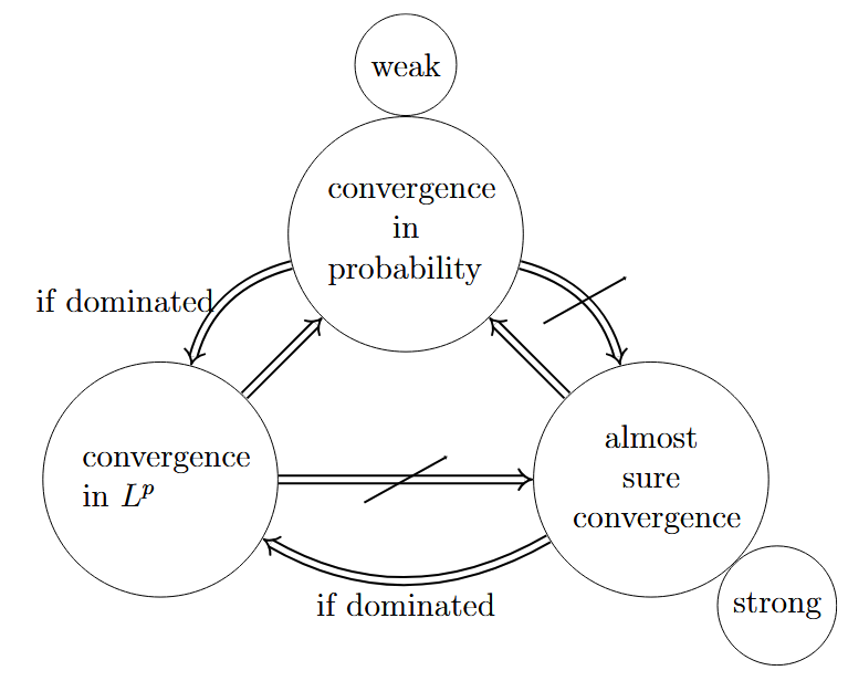
Theorem:

(a) If $p_1 < p_2$, then $X_n \to X$ in $L^{p_2}$ implies $X_n \to X$ in $L^{p_1}$.

(b) $X_n \to X$ in $L^p$ or almost surely implies $X_n \to X$ in probability.

(c) Suppose there exists $Y \in L^p$ such that $|X_n| \leq Y$ for all $n$. If $X_n \to X$ in probability and $X \in L^p$, then $X_n \to X$ in $L^p$.

proof:

$\square$

Corollary: If $X_n \to X’$ in $L^p$ and $X_n \to X’’$ almost surely, then $X’ = X’’$ a.e. (i.e. $P(X’ = X’’) = 1$).

proof:

It follows from the Theorem that $X_n \to X$ and $X_n \to X’’$ in probability, since the limit is unique, one has $X’ = X’’$ a.e.$\square$

Conditional Expectation

Definitions

Definition:

Let $(\Omega, \mathcal{F}_0, P)$ be a probability space. Let $X : \Omega \to [-\infty, +\infty]$ be an $(\mathcal{F}_0, \mathcal{B}([-\infty,+\infty]))$-measurable random variable with $\mathbb{E}[|X|] < \infty$ or $X \geq 0$, and let $\mathcal{F} \subseteq \mathcal{F}_0$ be a $\sigma$-algebra.

The conditional expectation $\mathbb{E}[X \mid \mathcal{F}]$ of $X$ given $\mathcal{F}$ is a random variable $Y : \Omega \to [-\infty, +\infty]$ with the following properties:

(C1) $Y$ is $(\mathcal{F}, \mathcal{B}([-\infty,+\infty]))$-measurable.
(C2)
$\int_A X \, dP = \int_A Y \, dP \quad \forall A \in \mathcal{F}$

If $\mathbb{E}[|X|] < \infty$, then $\mathbb{E}[X \mid \mathcal{F}]$ is almost surely finite. Every random variable fulfilling (C1) and (C2) is called a version of $\mathbb{E}[X \mid \mathcal{F}]$.

Definition:

$\mathbb{E}[X \mid Y]:= \mathbb{E}[X \mid \sigma(Y)]$

Theorem:

The conditional expectation exists and is almost surely unique.

Proporties

Theorem:

1. $X$ $\mathcal{F}$-measurable $\Longrightarrow$ $\mathbb{E}[X\mid \mathcal{F}] = X$ almost surely.

2. $\sigma(X)$ and $\mathcal{F}$ are independent $\Longrightarrow$ $\mathbb{E}[X \mid \mathcal{F}] = \mathbb{E}[X]$ almost surely.

Theorem:

1. Linearity: For $a \in \mathbb{R}$,

$\mathbb{E}[aX + Y \mid \mathcal{F}] = a \mathbb{E}[X \mid \mathcal{F}] + \mathbb{E}[Y \mid \mathcal{F}] \quad \text{almost surely.}$

2. Monotonicity: $X \leq Y \quad \Longrightarrow \quad \mathbb{E}[X \mid \mathcal{F}] \leq \mathbb{E}[Y \mid \mathcal{F}]$ almost surely.

3. Monotone convergence: $X_n \geq 0$, $X_n \uparrow X \quad \Longrightarrow \quad \mathbb{E}[X_n \mid \mathcal{F}] \uparrow \mathbb{E}[X \mid \mathcal{F}]$ almost surely.

Theorem:

$\mathbb{E}[\mathbb{E}[X \mid \mathcal{F}] = \mathbb{E}[X]$

Theorem:

If $X$ is $\mathcal{F}$-measurable, $\mathbb{E}[|XY|] < \infty$ and $\mathbb{E}[|Y|] < \infty$, then

$\mathbb{E}[XY \mid \mathcal{F}] = X \mathbb{E}[Y \mid \mathcal{F}] \quad \text{almost surely}.$

This holds also if $X \geq 0$ and $Y \geq 0$.

Theorem (“The smaller $\sigma$-algebra wins”) : Let $\mathcal{F}_1, \mathcal{F}_2$ be $\sigma$-algebras satisfying $\mathcal{F}_1 \subseteq \mathcal{F}_2$,$X$ be random variable. Then

$\mathbb{E}[\mathbb{E}[X \mid \mathcal{F}_1] \mid \mathcal{F}_2] = \mathbb{E}[\mathbb{E}[X \mid \mathcal{F}_2] \mid \mathcal{F}_1]= \mathbb{E}[X \mid \mathcal{F}_1]$

almost surely.